
The Rise of Deep Learning 🔥
While artificial intelligence has been a hot topic among scientists in the 1950s to 1980s, the industry only started to take the world by storm in the last two decades.
Its recent gain in popularity can be accredited to breakthroughs in deep learning made by various academics, notably Geoffrey Hinton from the University of Toronto, as well as the exponential increases in computational power and the amount of available data in the world.

Deep learning is a subset of artificial intelligence that uses algorithms modelled after the human brain called neural networks.
The Basic Structure of a Neural Network 🧱
Essentially, neural networks learn relationships between input variables and output variables. Given enough data about a set of x and y, neural networks learn to map accurately from x to y.
Neural networks are composed of layers of interconnected processing elements. These elements are called ‘nodes’ or ‘neurons’, and they work together to solve complex problems. The nodes are structured into layers split into three main types: input, hidden, and output layers.

The nodes in the input layer receive input values, those in the hidden layers perform hidden calculations and the nodes in the output layer return the network’s predictions.
Let’s say we are training our network to recognize handwritten digits in a 16×16 pixel grid. To receive inputs from this image, we would assign 16×16 or 256 nodes to the input layer. Starting from the top left corner of the image, each pixel is represented by one node.

An input node would contain some numeric value between -1 and 1 to represent the brightness of its corresponding pixel, where -1 is dark and 1 is white. As these values are inputted into the network, they are propagated forward from one layer of neurons to the next.
After they pass through a series of calculations in the hidden layers, we expect to receive ten outputs, where each output node represents a digit from 0 to 9. Hypothetically, if we show the network a handwritten ‘4’, the network should classify our image as a ‘4’. Mathematically, the node corresponding to the digit ‘4’ would return the highest value in the output layer.
Altogether, the nodes in the input layer receive input values, those in the hidden layers perform calculations and those in the output layer return predictions.
Understanding A Single Node! ☝️️
The big question is, how does our neural network model relationships? To understand the workings of a neural network, we must first understand the function of a single node in the hidden layers. We can compare the function of a single node to that of an iconic model in statistics — linear regression.
Linear regression can be defined as an attempt to model a linear relationship. Imagine you are given a set of data containing two quantitative variables:

If you were to plot the students’ marks against the number of hours they studied in a scatterplot, you would expect to find a positive linear relationship.
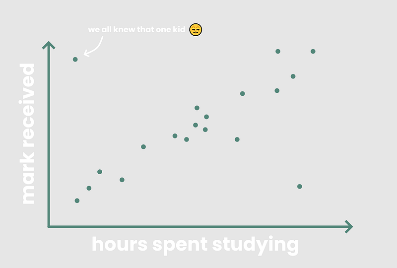
Typically, the longer a student spends studying, the likelier they are to score higher on the test. What linear regression tries to do is that it models this linear relationship by drawing a line of best fit through the points on the scatterplot, called a linear model. A linear model is basically a line, y = mx + b, that passes through as much of the data as possible.
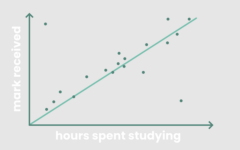
The ideal linear model would be one that minimizes the error between the students’ actual marks and the marks predicted by the model, or the error between the model’s actual y-values in and its predicted y-values.
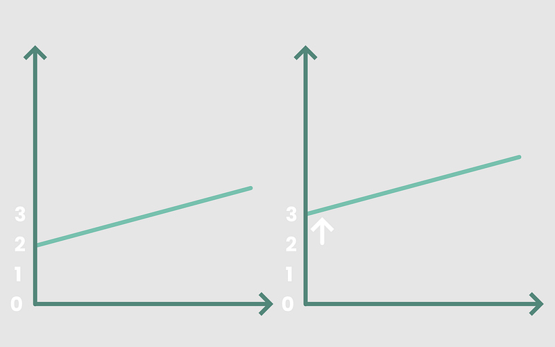
Let’s take a closer look at the math. In a linear model, an input x is multiplied by constant m. An input b is then added, which is called the ‘intercept’. These inputs are then summed together to get our output, y.
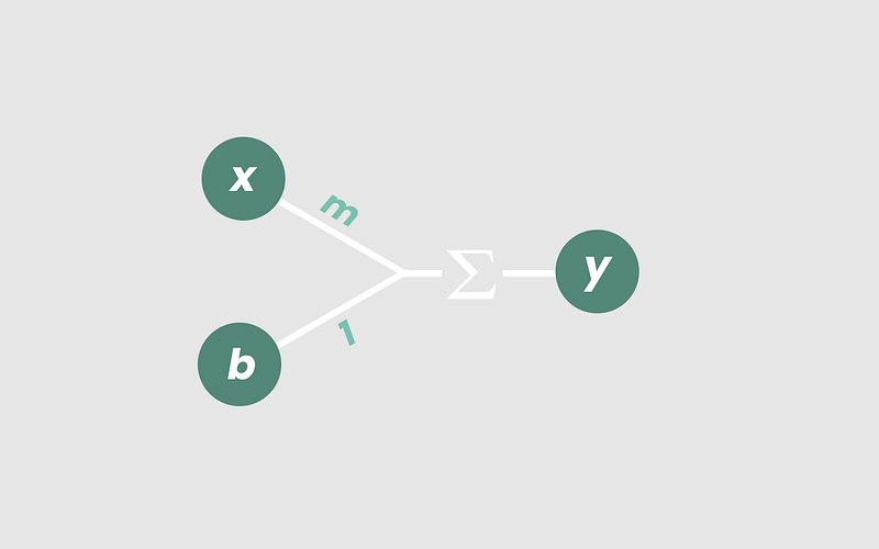
The resulting line, y = mx + b, models the relationship between x and y. If we were to modify the value of the inputs, we expect a different line. For instance, changing the constant b from 2 to3 means shifting our line up so that it intercepts the y-axis at y = 3 instead of y = 2.
The reason why I spent so long reviewing grade 9 math with you is simple. A single neuron works the exact same way!
In a neuron, an input x₁ is multiplied by a weight, w₁. After our input x₁ is multiplied by w₁, we call it a ‘weighted input’. A constant b₁ is then added — it behaves similarly to the y-intercept in a linear model, and is called the ‘bias’. The weighted input and bias are then summed together to get our output, v₀.

And there we go! A basic neuron.
Once again, we can adjust the value of v₀ by tweaking the weight, w₁, or the bias, b₁. If we modify either of the two parameters, we would again expect to see a different linear model.
But what if we add more inputs? 🤔
A linear regression model minimizes the error between an input’s actual output and the model’s predicted output. Similarly, the ideal neural network tries to do just that.
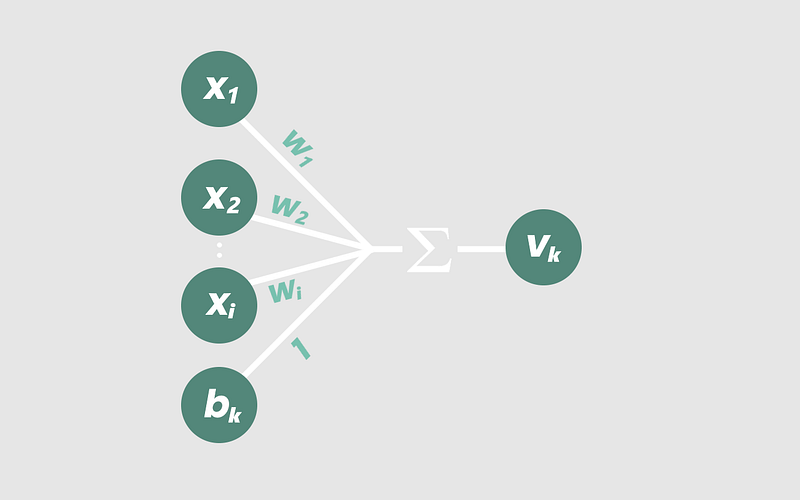
What sets a neuron apart from a linear regression model is that a neuron can receive several weighted inputs, where the number of inputs is denoted by the letter i. Here’s what that looks like mathematically:
vₖ = x₁ × w₁ + x₂ × w₂ . . . + xᵢ × wᵢ + bₖ.
In other words, the output vₖ of any neuron is just the summation, over all values of i, of xᵢ × wᵢ, added to bₖ.
But imagine we had seventeen x inputs… wouldn’t it be extremely tedious to write them all out by hand? That’s why we use mathematical notation to condense the function to a simple, elegant equation:
vₖ = ∑ ( xᵢ × wᵢ ) + bₖ
The subscript ₖ represents the current layer of the node, starting from the input layer.
Isn’t that much nicer to look at? Visually, here’s what our new node looks like:
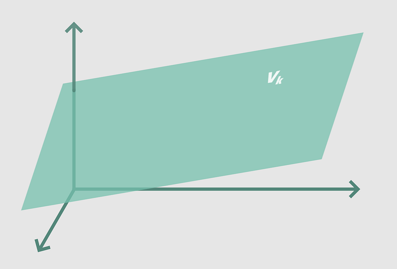
As we increase our number of inputs, our equation starts to model linear relationships in increasingly higher dimensions. For instance, a node with three weighted inputs
vₖ = x₁ × w₁ + x₂ × w₂ + x₃ × w₃ + b₁
would yield the three dimensional equivalent of a line: a plane.
If we were to add more inputs to the node, we would increase the number of dimensions modelled by the node’s equation. It would eventually model an i-dimensional hyperplane — the equivalent of a straight line in i-dimensional space.
(Don’t worry if you can’t visualize that, because neither can I 😂).
Thus far, the function we’ve outlined applies to just a single node in one layer of a neural network. Each node’s output, vₖ, becomes the input for every node in the next layer.
This process is then repeated across every single node in every layer of the neural network! I know, it’s a bit hard to wrap your mind around such high dimensional complexity. We are, unfortunately, only limited to our three-dimensional brains—for now, at least. But that’s a story for another time.
Accounting for Non-Linearity 〰️
Keep in mind, if we take our current layered neural network and set all the weights and biases randomly, the resulting weighted function at the output nodes would still be straight and linear. No matter how we combine our weights and sums, we will always get a linear model… that’s just how the math works out so far.
While it might be fun to model linear relationships, that’s not incredibly useful. We want our neural network to account for complex, nonlinear relationships.
Thus, we are going to modify the linear equation at each node to add some nonlinearity to our network, using what we call an ‘activation function.’
Think of this as a function that ‘activates’ our neural network, as its purpose is to enable our network to go from modelling linear i-dimensional hyperplanes to modelling nonlinear i-dimensional functions.
One popular activation function is the logistic curve, also known as the sigmoid function:
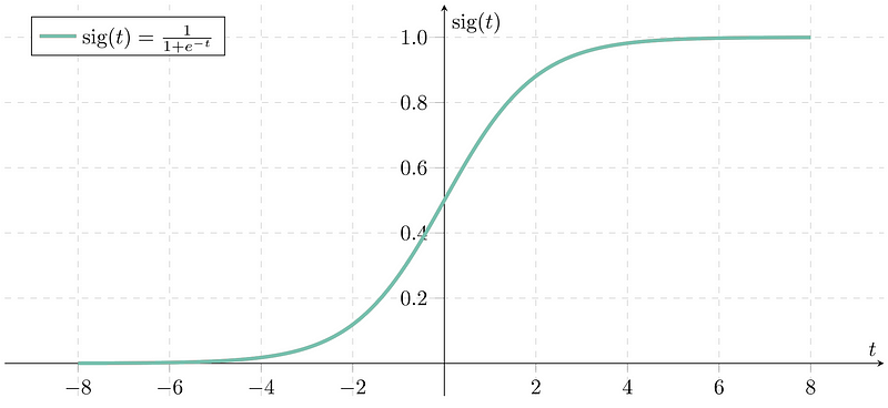
This function ‘squishes’ our weighted sums so that no matter how high or low they get, they will always end up between 0 and 1. After passing our existing equation at each node through the sigmoid function, our modified equation then becomes:
yₖ = σ ( vₖ )
or
yₖ = σ ( ∑ ( xᵢ × wᵢ ) + bₖ )
Adding this component to our diagram, we now have:

And now, our node is actually complete!
The sigmoid function allows our node to account for the interactive effects and non-linear relationships between multiple inputs. When connected with all the other nodes in the network, our neural network gains the ability to model complex nonlinear i-dimensional relationships.
A neural network that models the relationship between just three inputs might end up looking something like this:

But something as simple as the nonlinear plane visualized above could be computed by humans. We don’t really need a neural network for modelling functions in 3D space.
Neural networks become extremely useful when we start manipulating more and more variables and getting into higher and higher dimensions. I mean, how the hell would we come up with a model that accurately maps between thousands of variables?!
The answer is — we don’t. That’s what neural networks are for!
Let me reiterate:
As weighted inputs are added together and passed through an activation function at every node, neural networks gain the ability to model nonlinear i-dimensional relationships.
That’s why neural networks are so useful.
Since we can modify the weights and biases of every node, our neural network should now, in theory, be able to learn and model any relationship between any number of variables.
Only Now Do We Start to Train Our Network! 🏋️
With all this in mind, we start training our neural network with a random set of weights and biases at each node.
As we feed the network a large set of data and training examples containing both the inputs and the correct outputs, the network attempts to map inputs to their corresponding outputs.
The node in the output layer that is the most ‘active’, which is another way of saying that it returns a higher value than the weighted sums in the other output nodes, is the neural network’s choice for the ‘correct answer’ for a given set of inputs.
So Many Mistakes! 😬
Obviously, since we start with random weights and biases at each node, the network’s predictions will not be accurate from the get-go. This is why we need to train the network.
We show the network the correct answers for our training examples, and we basically tell the network to see how close its predictions are to the correct answers each time. We do this by calculating how much error we have in our output using a loss function:
Error = ½ × (Actual output — Predicted Output)²
Our goal is to minimize error to increase the network’s accuracy. A simple way to visualize this process is to imagine graphing error as a parabolic function that opens upwards, where the trough at the bottom represents the minimum error.
We use a method called gradient descent to minimize the derivative of our point on this loss function. This is a fancy way of saying, if we were to draw a line that is tangent to our point, we want its slope to be as small as possible.
The only point where the slope of the tangent line of our parabola would be 0 is at the bottom-most point, where loss is minimized. Knowing the derivative of our point on our loss function is incredibly useful because the smaller it becomes, the less the error.
Hence, the gradient descent function helps us to minimize loss by shifting our neural network’s error point down to a local minimum of the loss function.
In practice, our loss function won’t be a two-variable parabola, since most neural networks have more than just two inputs and therefore more than two variables.
Instead, the loss function would resemble hills and valleys in multidimensional space. The gradient descent function therefore reduces error by minimizing the ‘gradient’, or multivariable derivative, of our point on the loss function.
So rather than lowering our loss on a parabola, imagine the process of gradient descent as rolling a ball down a hill, where the ball represents the amount of error in our neural network.

In brief, gradient descent allows the network to calculate whether its output needs to be more positive or negative given a set of inputs so that the network’s overall accuracy improves when making predictions.
Fix Them Mistakes! 😤
Once the error has been calculated by the loss function, the weights and biases in the network are then modified to minimize error. This is done using a method called back-propagation:
W(k+1) = W(k) — (Learning Rate) × (Gradient Descent Applied to Error)
where W(k+1) represents a new weight and W(k) represents our current weight.
The back-propagation function propagates the error from the output layer backwards through every layer in the network. It essentially allows us to modify the value of every weight between the nodes in our neural network so that some nodes become more ‘active’ than others.
These modifications are made with the aim of minimizing the loss, or error, in our neural network. After numerous iterations of training, loss is minimized and our neural network becomes increasingly accurate at its job, whether it be recognizing handwritten digits or recommending your next YouTube video.
Key Takeaways 🔑
→ Neural networks learn relationships between input variables and output variables.
→ Given enough data to train on, neural networks learn to map accurately from x to y.
→ Neural networks are composed of input, hidden, and output layers.
→ The function of a single node can be compared to linear regression, where each node has a set of weights and biases.
→ What sets a neuron apart from a linear regression model is that a node can receive several weighted inputs and that each node in one layer feeds into the nodes in the next layer. This characteristic is what allows neural networks to model extremely complex relationships between dozens, hundreds, or thousands of variables.
→ We use activation functions to account for non-linearity in relationships between variables.
→ Gradient descent is used to identify and minimize the loss in neural networks and works similarly to a ball rolling down hills and valleys.
→ Once the loss is identified, it is minimized through back-propagation; the error at the output layer is propagated backwards using the chain rule from calculus so that the weights and biases are tweaked in each layer.